 |
|
|
| |
|
|
The aim of this tutorial is to train users to perform metadynamics simulations with PLUMED, analyze the results, calculating free-energies as a function of the collective variables used, and estimating the associated error.
Once this tutorial is completed students will be able to:
The TARBALL for this project contains the following files:
This tutorial has been tested on a pre-release version of version 2.4. However, it should not take advantage of 2.4-only features, thus should also work with version 2.3.
We have seen that PLUMED can be used to compute collective variables. However, PLUMED is most often use to add forces on the collective variables. To this aim, we have implemented a variety of possible biases acting on collective variables. The complete documentation for all the biasing methods available in PLUMED can be found at the Bias page. In the following we will see how to build an adaptive bias potential with metadynamics. Here you can find a brief recap of the metadynamics theory.
In metadynamics, an external history-dependent bias potential is constructed in the space of a few selected degrees of freedom \( \vec{s}({q})\), generally called collective variables (CVs) [64]. This potential is built as a sum of Gaussian kernels deposited along the trajectory in the CVs space:
\[ V(\vec{s},t) = \sum_{ k \tau < t} W(k \tau) \exp\left( -\sum_{i=1}^{d} \frac{(s_i-s_i({q}(k \tau)))^2}{2\sigma_i^2} \right). \]
where \( \tau \) is the Gaussian deposition stride, \( \sigma_i \) the width of the Gaussian for the \(i\)th CV, and \( W(k \tau) \) the height of the Gaussian. The effect of the metadynamics bias potential is to push the system away from local minima into visiting new regions of the phase space. Furthermore, in the long time limit, the bias potential converges to minus the free energy as a function of the CVs:
\[ V(\vec{s},t\rightarrow \infty) = -F(\vec{s}) + C. \]
In standard metadynamics, Gaussian kernels of constant height are added for the entire course of a simulation. As a result, the system is eventually pushed to explore high free-energy regions and the estimate of the free energy calculated from the bias potential oscillates around the real value. In well-tempered metadynamics [8], the height of the Gaussian is decreased with simulation time according to:
\[ W (k \tau ) = W_0 \exp \left( -\frac{V(\vec{s}({q}(k \tau)),k \tau)}{k_B\Delta T} \right ), \]
where \( W_0 \) is an initial Gaussian height, \( \Delta T \) an input parameter with the dimension of a temperature, and \( k_B \) the Boltzmann constant. With this rescaling of the Gaussian height, the bias potential smoothly converges in the long time limit, but it does not fully compensate the underlying free energy:
\[ V(\vec{s},t\rightarrow \infty) = -\frac{\Delta T}{T+\Delta T}F(\vec{s}) + C. \]
where \( T \) is the temperature of the system. In the long time limit, the CVs thus sample an ensemble at a temperature \( T+\Delta T \) which is higher than the system temperature \( T \). The parameter \( \Delta T \) can be chosen to regulate the extent of free-energy exploration: \( \Delta T = 0\) corresponds to standard MD, \( \Delta T \rightarrow\infty\) to standard metadynamics. In well-tempered metadynamics literature and in PLUMED, you will often encounter the term "bias factor" which is the ratio between the temperature of the CVs ( \( T+\Delta T \)) and the system temperature ( \( T \)):
\[ \gamma = \frac{T+\Delta T}{T}. \]
The bias factor should thus be carefully chosen in order for the relevant free-energy barriers to be crossed efficiently in the time scale of the simulation. Additional information can be found in the several review papers on metadynamics [63] [9] [101]. To learn more: Summary of theory
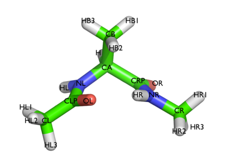
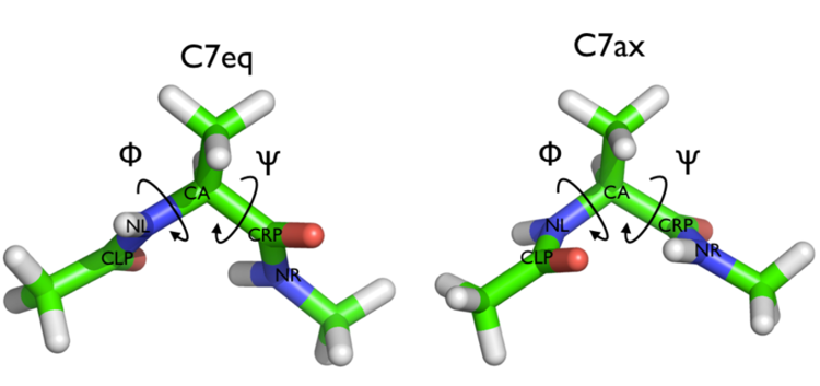
We will play with a toy system, alanine dipeptide simulated in vacuo using the AMBER99SB-ILDN force field (see Fig. trieste-4-ala-fig). This rather simple molecule is useful to benchmark data analysis and free-energy methods. This system is a nice example because it presents two metastable states separated by a high free-energy barrier. It is conventional use to characterize the two states in terms of Ramachandran dihedral angles, which are denoted with \( \Phi \) and \( \Psi \) in Fig. trieste-4-transition-fig .
In this exercise we will setup and perform a well-tempered metadynamics run using the backbone dihedral \( \phi \) as collective variable. During the calculation, we will also monitor the behavior of the other backbone dihedral \( \psi \).
Here you can find a sample plumed.dat file that you can use as a template. Whenever you see an highlighted FILL string, this is a string that you should replace.
# Compute the backbone dihedral angle phi, defined by atoms C-N-CA-C
phi: TORSION ATOMS=__FILL__
# Compute the backbone dihedral angle psi, defined by atoms N-CA-C-N
psi: TORSION ATOMS=__FILL__

# Activate well-tempered metadynamics in phi
metad: __FILL__ ARG=__FILL__ ...
# Deposit a Gaussian every 500 time steps, with initial height equal to 1.2 kJ/mol
PACE=500 HEIGHT=1.2
# the bias factor should be wisely chosen
BIASFACTOR=__FILL__
# Gaussian width (sigma) should be chosen based on CV fluctuation in unbiased run
SIGMA=__FILL__
# Gaussians will be written to file and also stored on grid
FILE=HILLS GRID_MIN=-pi GRID_MAX=pi
...

# Print both collective variables and the value of the bias potential on COLVAR file
PRINT ARG=__FILL__ FILE=COLVAR STRIDE=10
The syntax for the command METAD is simple. The directive is followed by a keyword ARG followed by the labels of the CVs on which the metadynamics potential will act. The keyword PACE determines the stride of Gaussian deposition in number of time steps, while the keyword HEIGHT specifies the height of the Gaussian in kJ/mol. For each CVs, one has to specify the width of the Gaussian by using the keyword SIGMA. Gaussian will be written to the file indicated by the keyword FILE.
In this example, the bias potential will be stored on a grid, whose boundaries are specified by the keywords GRID_MIN and GRID_MAX. Notice that you can provide either the number of bins for every collective variable (GRID_BIN) or the desired grid spacing (GRID_SPACING). In case you provide both PLUMED will use the most conservative choice (highest number of bins) for each dimension. In case you do not provide any information about bin size (neither GRID_BIN nor GRID_SPACING) and if Gaussian width is fixed, PLUMED will use 1/5 of the Gaussian width as grid spacing. This default choice should be reasonable for most applications.
Once your plumed.dat file is complete, you can run a 10-ns long metadynamics simulations with the following command
> gmx mdrun -s topol.tpr -nsteps 5000000 -plumed plumed.dat
During the metadynamics simulation, PLUMED will create two files, named COLVAR and HILLS. The COLVAR file contains all the information specified by the PRINT command, in this case the value of the CVs every 10 steps of simulation, along with the current value of the metadynamics bias potential. We can use gnuplot to visualize the behavior of the CV during the simulation, as reported in the COLVAR file:
gnuplot> p "COLVAR" u 1:2
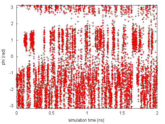
By inspecting Figure trieste-4-phi-fig, we can see that the system is initialized in one of the two metastable states of alanine dipeptide. After a while (t=0.1 ns), the system is pushed by the metadynamics bias potential to visit the other local minimum. As the simulation continues, the bias potential fills the underlying free-energy landscape, and the system is able to diffuse in the entire phase space.
The HILLS file contains a list of the Gaussian kernels deposited along the simulation. If we give a look at the header of this file, we can find relevant information about its content:
#! FIELDS time phi sigma_phi height biasf
#! SET multivariate false
#! SET min_phi -pi
#! SET max_phi pi
The line starting with FIELDS tells us what is displayed in the various columns of the HILLS file: the simulation time, the instantaneous value of \( \phi \), the Gaussian width and height, and the bias factor. We can use the HILLS file to visualize the decrease of the Gaussian height during the simulation, according to the well-tempered recipe:
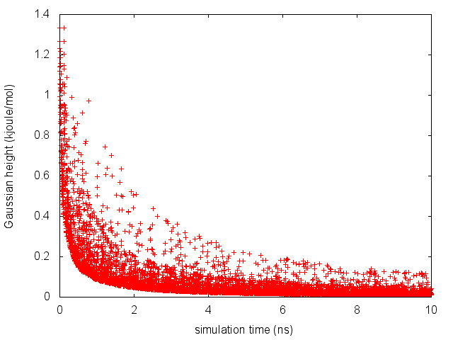
If we look carefully at the scale of the y-axis, we will notice that in the beginning the value of the Gaussian height is higher than the initial height specified in the input file, which should be 1.2 kJ/mol. In fact, this column reports the height of the Gaussian scaled by the pre-factor that in well-tempered metadynamics relates the bias potential to the free energy.
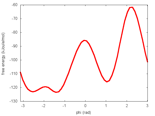
One can estimate the free energy as a function of the metadynamics CVs directly from the metadynamics bias potential. In order to do so, the utility sum_hills should be used to sum the Gaussian kernels deposited during the simulation and stored in the HILLS file.
To calculate the free energy as a function of \( \phi \), it is sufficient to use the following command line:
plumed sum_hills --hills HILLS
The command above generates a file called fes.dat in which the free-energy surface as function of \( \phi \) is calculated on a regular grid. One can modify the default name for the free energy file, as well as the boundaries and bin size of the grid, by using the following options of sum_hills :
--outfile - specify the outputfile for sumhills
--min - the lower bounds for the grid
--max - the upper bounds for the grid
--bin - the number of bins for the grid
--spacing - grid spacing, alternative to the number of bins
The result should look like this:
To assess the convergence of a metadynamics simulation, one can calculate the estimate of the free energy as a function of simulation time. At convergence, the reconstructed profiles should be similar. The option --stride should be used to give an estimate of the free energy every N Gaussian kernels deposited, and the option --mintozero can be used to align the profiles by setting the global minimum to zero. If we use the following command line:
plumed sum_hills --hills HILLS --stride 100 --mintozero
one free energy is calculated every 100 Gaussian kernels deposited, and the global minimum is set to zero in all profiles. The resulting plot should look like the following:
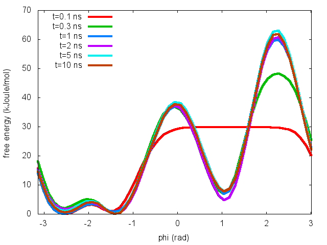
These two qualitative observations:
suggest that the simulation most likely converged.
In this exercise, we will run a well-tempered metadynamics simulation on alanine dipeptide in vacuum, this time using as CV the backbone dihedral \( \psi \). Please complete the template plumed.dat file used in the previous exercise to run this calculation.
Once your plumed.dat file is complete, you can run a 10-ns long metadynamics simulations with the following command
> gmx mdrun -s topol.tpr -nsteps 5000000 -plumed plumed.dat
As we did in the previous exercise, we can use COLVAR to visualize the behavior of the CV during the simulation. Here we will plot at the same time the evolution of the metadynamics CV \( \psi \) and of the other dihedral \( \phi \).
gnuplot> p "COLVAR" u 1:2, "" u 1:3
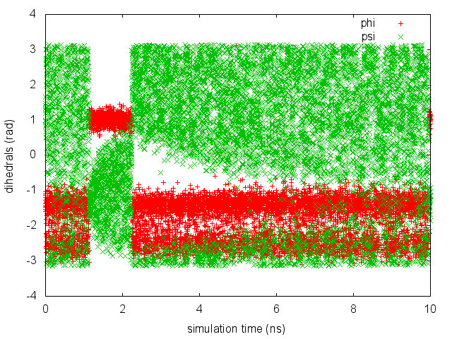
By inspecting Figure trieste-4-metad-psi-phi-fig, we notice that something different happened compared to the previous exercise. At first the behavior of \( \psi \) looks diffusive in the entire CV space. However, around t=1 ns, \( \psi \) seems trapped in a region of the CV space in which it was previously diffusing without problems. The reason is that the non-biased CV \( \phi \) after a while has jumped into a different local minima. Since \( \phi \) is not directly biased, one has to wait for this (slow) degree of freedom to equilibrate before the free energy along \( \psi \) can converge.
Try to repeat the analysis done in the previous exercise, i.e. calculate the estimate of the free energy as a function of time, first step to assess the convergence of this metadynamics simulation.
In this exercise, we will calculate the error associated to the free-energy reconstructed by a well-tempered metadynamics simulation. The free energy and the errors will be calculated using the block-analysis technique explained in a previous lesson (Trieste tutorial: Averaging, histograms and block analysis). The procedure can be used to estimate the error in the free-energy as a function of the collective variable(s) used in the metadynamics simulation, or for any other function of the coordinates of the system.
First, we will calculate the "un-biasing" weights associated to each conformation sampled during the metadynamics run. In order to calculate these weights, we can use either of these two approaches:
1) Weights are calculated by considering the time-dependence of the metadynamics bias potential [103];
2) Weights are calculated using the metadynamics bias potential obtained at the end of the simulation and assuming a constant bias during the entire course of the simulation [24].
In this exercise we will use the umbrella-sampling-like reweighting approach (Method 2).
To calculate the weights, we need to use the PLUMED driver utility and read the HILLS file along with the GROMACS trajectory file produced during the metadynamics simulation. Let's consider the metadynamics simulation carried out in Exercise 1. We need to prepare the plumed.dat input file to use in combination with driver. Here you can find a sample plumed.dat file that you can use as a template. Whenever you see an highlighted FILL string, this is a string that you should replace.
# Read old Gaussians deposited on HILLS file
RESTART
# Compute the backbone dihedral angle phi, defined by atoms C-N-CA-C
phi: TORSION ATOMS=__FILL__
# Compute the backbone dihedral angle psi, defined by atoms N-CA-C-N
psi: TORSION ATOMS=__FILL__

# Activate well-tempered metadynamics in phi
metad: __FILL__ ARG=__FILL__ ...
# Set the deposition stride to a large number
PACE=10000000 HEIGHT=1.2 BIASFACTOR=__FILL__
# Gaussian width (sigma) should be chosen based on CV fluctuation in unbiased run
SIGMA=__FILL__
# Gaussians will be read from file and stored on grid
FILE=HILLS GRID_MIN=-pi GRID_MAX=pi
...

# Print both collective variables and the value of the bias potential on COLVAR file
PRINT ARG=__FILL__ FILE=COLVAR STRIDE=1
Once your plumed.dat file is complete, you can use the driver utility to back-calculated the quantities needed for the error calculation
plumed driver --plumed plumed.dat --mf_xtc traj_comp.xtc
The COLVAR file produced by driver should look like this:
#! FIELDS time phi psi metad.bias
#! SET min_phi -pi
#! SET max_phi pi
#! SET min_psi -pi
#! SET max_psi pi
 0.000000 0.907347 -0.144312 103.117323
 1.000000 0.814296 -0.445819 100.974351
 2.000000 1.118951 -0.909782 104.329630
 3.000000 1.040781 -0.991788 104.559590
 4.000000 1.218571 -1.020024 102.744053
Please check your plumed.dat file if your output looks different! Once the final bias has been evaluated on the entire metadynamics simulations, we can easily calculate the "un-biasing weights" using the umbrella-sampling-like approach:
# find maximum value of bias
bmax=`awk 'BEGIN{max=0.}{if($1!="#!" && $4>max)max=$4}END{print max}' COLVAR`

# print phi values and weights
awk '{if($1!="#!") print $2,exp(($4-bmax)/kbt)}' kbt=2.494339 bmax=$bmax COLVAR > phi.weight
If you inspect the phi.weight file, you will see that each line contains the value of the dihedral \( \phi \) along with the corresponding weight:
0.907347 0.0400579
0.814296 0.0169656
1.118951 0.0651276
1.040781 0.0714174
1.218571 0.0344903
1.090823 0.0700568
1.130800 0.0622998
At this point we can apply the block-analysis technique we have learned in the Trieste tutorial: Averaging, histograms and block analysis tutorial to calculate for different block sizes the average free-energy and the error. For your convenience, you can use the do_block_fes.py python script to read the phi.weight file and produce the desired output. We use a bash loop to use block sizes ranging from 1 to 1000:
for i in `seq 1 10 1000`; do python3 do_block_fes.py phi.weight 1 -3.141593 3.018393 51 2.494339 $i; done
For each value of block length N, you will obtain a separate fes.N.dat file, containing the value of the \( \phi \) variable on a grid, the average free-energy, and the associated error (in kJ/mol):
   -3.141593       23.184653     0.080659
   -3.018393       17.264462     0.055181
   -2.895194       13.360259     0.047751
   -2.771994       10.772696     0.043548
   -2.648794        9.403544     0.042022
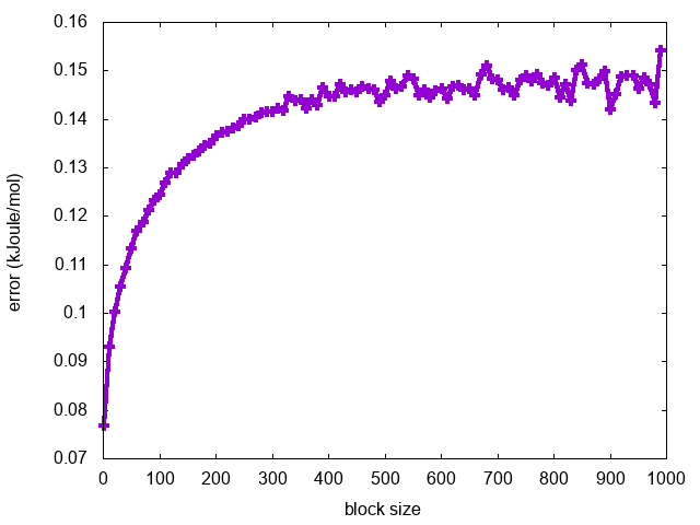
Finally, we can calculate the average error along the free-energy profile as a function of the block length:
for i in `seq 1 10 1000`; do a=`awk '{tot+=$3}END{print tot/NR}' fes.$i.dat`; echo $i $a; done > err.blocks
and visualize it using gnuplot:
gnuplot> p "err.blocks" u 1:2 w lp
As expected, the error increases with the block length until it reaches a plateau in correspondence of a dimension of the block that exceeds the correlation between data points (Fig. trieste-4-block-phi).
To complete this exercise, you should do the following:
What can we learn from this analysis about the convergence of the two metadynamics simulations and the quality of the collective variables chosen?
At this time, the most important question of this lecture becomes:
In summary, in this tutorial you should have learned how to use PLUMED to:
 1.8.14